Using Stable Baselines to train Autonomous Drones

The realm of unmanned aerial vehicles (UAVs) is experiencing a surge in interest, a trend driven by their increasing versatility and expanding roles in various sectors. Fresh from completing CS 285 at UC Berkeley, where I deep-dived into reinforcement learning (RL) algorithms, I find the application of these algorithms in drones particularly fascinating.
So, why the interest in UAVs? First of all, there are numerous labs at Berkeley researching the intersection between UAVs and RL, so I was hoping to gain some knowledge on this task. Beyond that, these vehicles are revolutionizing numerous fields, from aerial photography and agricultural monitoring to search and rescue operations and delivery services. Their ability to access hard-to-reach areas, collect high-resolution data, and perform tasks with increased efficiency and reduced human risk makes them invaluable assets. Furthermore, the advancement in drone technology, such as improved battery life, enhanced sensors, and more sophisticated navigation systems, continues to broaden their potential applications.
In this article, we'll explore how different RL algorithms can be applied to this rapidly evolving field of autonomous drones. Here's our roadmap:
- PyFlyt Environment Overview: I'll start by introducing PyFlyt, a simulation environment tailor-made for training autonomous drones. Rather than having to use real drones that require power and can get damaged, PyFlyt provides a safe and controlled simulation setting to experiment with RL algorithms, crucial for developing reliable drone control systems.
- Understanding Reinforcement Learning Algorithms: I'll provide a concise overview of various RL algorithms (A2C, PPO, DDPG, TD3, SAC). There will be a little bit of math here, but it won't be too necessary for understanding the rest of the article, so it can easily be skipped.
- Utilizing Stable Baselines Training: Central to our exploration is the application of the stable baseline implementations of these RL algorithms. For my class, I implemented many of these RL algorithms from the ground up with PyTorch, so going into this project I was excited to be able to black box the algorithms by just importing them and calling them (yes, it really was as easy as that!).
- Analyzing Results: The final section will present the outcomes of applying these algorithms within the PyFlyt environment.
PyFlyt Environment
PyFlyt is a Python package designed for the simulation and control of aerial vehicles . It offers functionalities for simulating flight and implementing various control algorithms. This package facilitates the testing and development of drone control systems in a simulated environment, which is essential for safe and efficient experimentation, especially when working with complex algorithms such as those used in reinforcement learning.
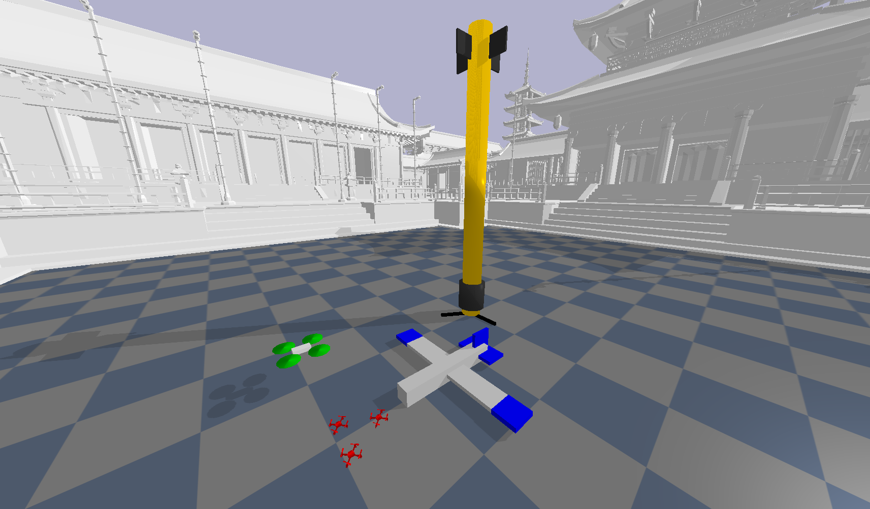
In this article, we focus on the QuadX-Waypoints-v1 environment, where a quadrotor drone is tasked with reaching a set of waypoints as fast as possible.
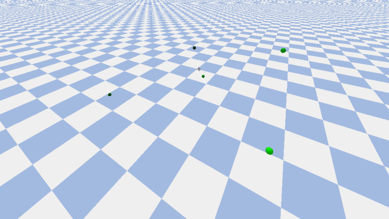
The actions available to the agent are \(v_p,v_q,v_r,T\) (angular rates and thrust). The goals are a set of \((x,y,z)\) triples (the waypoints in 3D space). The different shades of green of the waypoints in the above example indicate the order in which the agent must visit the waypoints.

Reinforcement Learning Algorithms
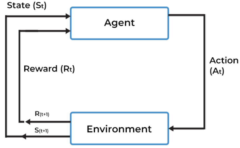
For this project, I applied the following RL algorithms: advantage actor critic (A2C), proximal policy optimization (PPO), deep deterministic policy gradient (DDPG), twin delayed deep deterministic policy gradient (TD3), and soft actor-critic (SAC). For my own learning, I'm going to attempt to explain (at a high level) what each of these algorithms are doing and how they work.
Advantage Actor Critic (A2C)
A2C separates the policy guide (actor) from the value estimate (critic). The actor decides the action, and the critic evaluates it. The 'advantage' part, \( A(s, a) = Q(s, a) - V(s) \), improves the policy by favoring actions that lead to better-than-average returns.
Proximal Policy Optimization (PPO)
PPO aims to improve policy learning by maintaining a balance between exploration and exploitation. It restricts the policy update step to avoid drastic changes, leading to more stable and efficient learning.
PPO modifies the objective function in two key ways:
- Ratio of New to Old Policy: This is represented by \( \frac{\pi_\theta(a|s)}{\pi_{\theta_{old}}(a|s)} \), where \( \pi_\theta \) is the new policy and \( \pi_{\theta_{old}} \) is the old policy. It measures how much the new policy deviates from the old.
- Clipped Surrogate Objective: To prevent large policy updates, PPO uses a clipped objective function. The clipping is done using the term \( \text{clip}\left(\frac{\pi_\theta(a|s)}{\pi_{\theta_{old}}(a|s)}, 1-\epsilon, 1+\epsilon\right) \), where \( \epsilon \) is a hyperparameter that defines the clip range. This clipping ensures the updated policy doesn't move too far from the old policy.
The objective function in PPO is a minimum of two terms: the unclipped and the clipped objectives. This design helps maintain a balance between exploration (trying new actions) and exploitation (using known good actions), leading to more stable and efficient policy learning.
Deep Deterministic Policy Gradient (DDPG)
DDPG is an algorithm for continuous action spaces. It uses a deep neural network to learn a deterministic policy and a Q-value function. It combines ideas from DPG (Deterministic Policy Gradient) and DQN (Deep Q-Network). The key components are:
- Actor Network: This network, \( \mu(s; \theta^\mu) \), outputs a deterministic action given the current state. It's updated to maximize the output of the critic network.
- Critic Network: Represented as \( Q(s, a; \theta^Q) \), it estimates the Q-value (the expected reward) of a state-action pair. It's updated based on the Temporal Difference (TD) error, similar to Q-learning.
- Target Networks: DDPG uses target networks for both the actor and critic to stabilize learning. These are slowly updated copies of the actor and critic networks.
- Experience Replay: Like DQN, DDPG uses a replay buffer to store and sample past experiences, aiding in efficient learning and breaking correlations between consecutive samples.
DDPG optimizes both networks using backpropagation, with the critic guiding the actor to choose actions that lead to higher future rewards.
Twin Delayed Deep Deterministic Policy Gradient (TD3)
An extension of DDPG, TD3 addresses DDPG's overestimation of Q-values. It introduces twin Q-networks and delayed policy updates, improving stability and performance in learning.
Soft Actor-Critic (SAC)
SAC is an off-policy algorithm that optimizes a stochastic policy in an entropy-augmented setting. It encourages exploration by adding an entropy term to the reward, leading to a balance between exploration and exploitation.
The key equation in SAC is:
\[ \max_{\pi} \mathbb{E}_{(s_t, a_t)\sim\pi}\left[r(s_t, a_t) + \alpha \mathcal{H}(\pi(\cdot|s_t))\right] \]
This objective function aims to maximize the expected sum of rewards \( r(s_t, a_t) \) and the entropy of the policy \( \mathcal{H}(\pi(\cdot|s_t)) \). The term \( \alpha \) is a temperature parameter that balances between reward maximization and entropy maximization. Entropy maximization encourages exploration by rewarding the policy for being uncertain or stochastic. This balance allows SAC to effectively explore the environment and learn robust policies.
Stable Baselines
It might be clear that implementing all of the above RL algorithms require a large number of technical details and design decisions. Thus, a Python library where all of these algorithms have already been implemented and can easily be used would be supremely useful. This is essentially what Stable Baselines is.
I found this YouTube series, Reinforcement Learning with Stable Baselines 3, to be very useful when first learning how to use this Python module. However, even without a tutorial, it's honestly so simple to use. If you have any experience with OpenAI's Gym, then it will be very intuitive to use.
My code was as simple as just two files (train.py and eval.py). The GitHub repository can be found here.
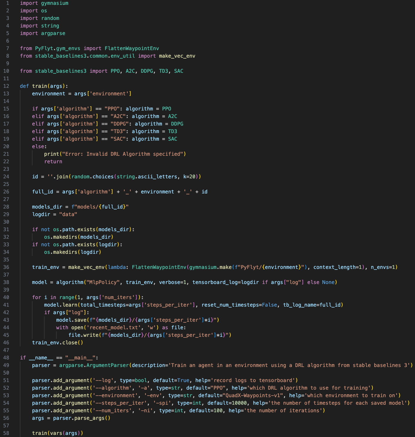
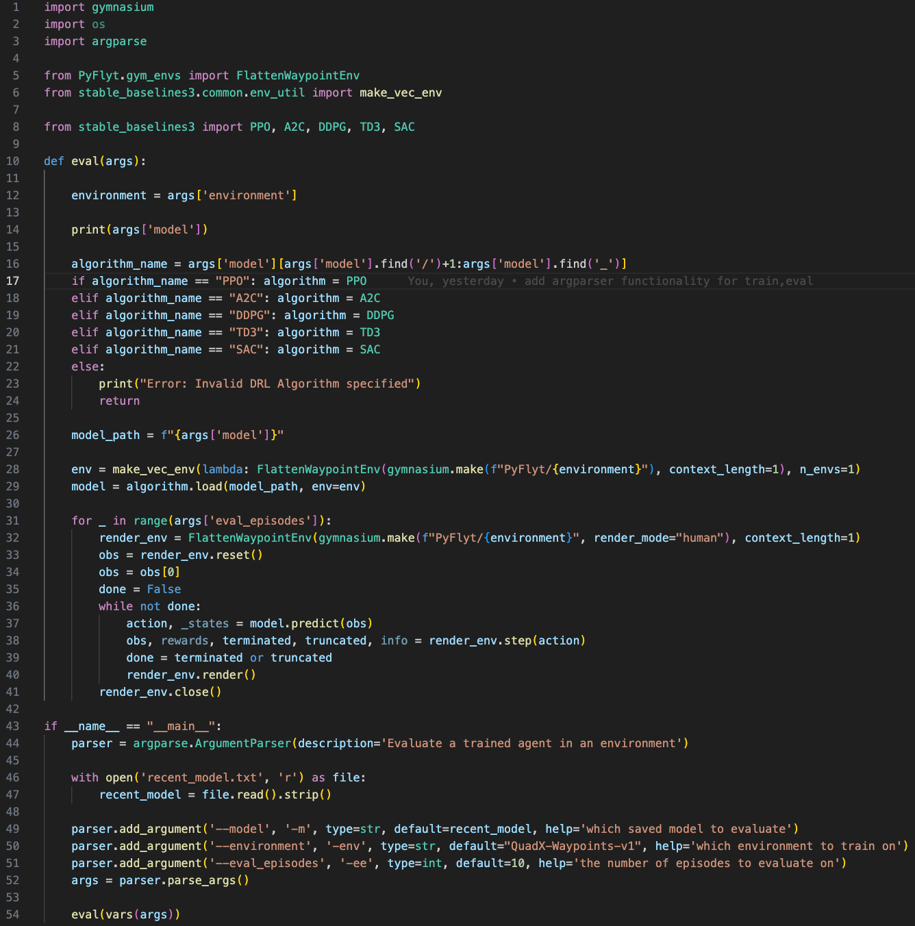
All 112 lines of code used to train the agent on 5 different RL algorithms using Stable Baselines3! (train.py is on the left and eval.py is on the right)
In train.py, Stable Baselines is used on line 38, 41, and 43, where the model is defined, trained, and saved. In eval.py, Stable Baselines is used on line 29, where the model is loaded. Without Stable Baselines, I would've had to rewrite these RL algorithms from scratch in separate files, increasing the time and complexity of this project by a lot.
Results
The best performing algorithms were PPO and TD3. An example of the corresponding algorithms being applied can be seen below.
PPO
TD3
Note that PPO took significantly less time and samples to reach its peak performance during training than TD3.
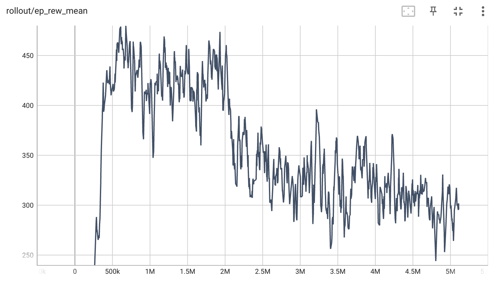

(training results for PPO on the left, TD3 on the right)
Conclusion
This was a short, but fun and interesting, project to practice my RL skills during the break. I enjoyed learning Stable Baselines and hope to use it in the future with custom environments. I'm thinking of returning to my Coup project with my newfound understanding of RL and Stable Baselines, and seeing if I can improve my results there.
Additionally, it could be interesting to apply my results on ACL to this environment, or even more generally, build some wrapper class or gym environment that automatically does some sort of curriculum learning. That's an idea I've been thinking about for awhile, and I'm not sure if one already exists.
As for the drone-specific continuations, it could be interesting to have more complex drones, different environmental effects (wind, noisy sensors, etc.), or moving targets.
I'm hoping to use my skills in RL and ML to get involved with research labs at Berkeley this upcoming semester!