
The Counterintuitive Mathematics of Random Walks

Recently, in a lecture for EECS 126, my professor told us an interesting fact about random walks. He left it as an exercise for us to understand, simply stating it without proof. This article presents my understanding of that fact.
A Random Walk Fact
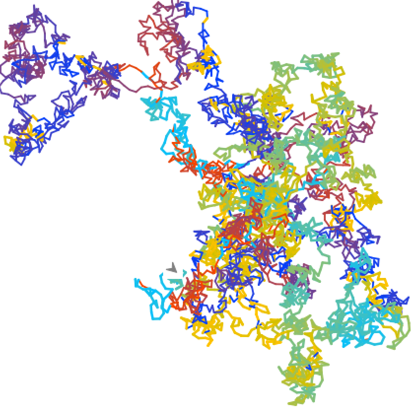
Imagine you live on the integer number line, \(\mathbb{Z}\) and start at some position \(X_0\). You live at the origin, \(0\), but did not start there. At each time step \(t\), your position \(X_t\) transitions to \(X_{t+1}\), which is one of your neighboring positions, with equal probability for each neighbor. This describes a random walk in one dimension. In this case, you are guaranteed to eventually reach your home. In fact, you are guaranteed to reach every possible position on the number line!
Now, play the same game but in two dimensions. That is, consider the two-dimensional grid of integers, \(\mathbb{Z}^2\). Again, performing a random walk guarantees that you will eventually reach your home, \((0,0)\).

One more time, let's play this game. Consider the three-dimensional grid of integers, \(\mathbb{Z}^3\). Same story: perform a random walk and see if you will eventually reach your home, \((0,0,0)\). Despite this being a guarantee in one and two dimensions, now you are not guaranteed to reach your home!
"A drunk man will find his way home, but a drunk bird may get lost forever."
When I first heard of this property of random walks, I was completely lost. How could simply increasing the dimensionality change what seemed to be an invariant property of randomness. With infinite time, shouldn't you be guaranteed to eventually reach your home? It's not like the cardinality of the world changed either (\(\mathbb{Z},\mathbb{Z}^2,\mathbb{Z}^3\) are all countably infinite sets). So, what changed?
To understand what's going on here, let's first formalize the problem with the notion of Markov chains. Along the way, we'll hopefully learn a lot of interesting probability theory concepts as we solve the puzzle.
Introduction to Markov Chains
Let \((X_n)_{n\in\mathbb{N}}\) be a sequence of random variables on a state space \(\mathcal{X}\). \((X_n)_{n\in\mathbb{N}}\) is a discrete-time Markov chain (DTMC) if it satisfies the Markov property:
\[\mathbb{P}(X_{n+1}=x_{n+1}|X_n=x_n,\ldots,X_0=x_0)=\mathbb{P}(X_{n+1}=x_{n+1}|X_n=x_n)\]
Oftentimes, \(\mathbb{P}(X_{n+1}=x_{n+1}|X_n=x_n)\) is written as \(P(x_n,x_{n+1})\), where \(P(\cdot,\cdot)\) is a set of nonnegative numbers such that for all \(x\in\mathcal{X}\),
\[\sum_{y\in\mathcal{X}}P(x,y)=1\]
The Markov property is often summarized by the statement "the past and future are conditionally independent given the present."
A Random Walk as a Markov Chain
Now, let's use the formal notion of Markov chains to define a \(d\)-dimensional random walk.
Let \(X_n\) denote our location at time step \(n\), where \(X_n=\sum_{i=1}^nS_i\), with \(S_i\) being the individual step taken at time step \(i\). That is, let each step \(S_i\) be i.i.d. drawn uniformly among the axis-aligned unit steps, so
\[\mathbb{P}(S_i=e_j)=\mathbb{P}(S_i=-e_j)=\frac{1}{2d},\]
where \(e_j\) is the \(j\)th unit vector. Thus, to describe the Markov chain, we have
\[P(x_n,x_{n+1})=\begin{cases}\frac{1}{2d} & \text{if $x_n,x_{n+1}$ are neighbors} \\ 0 & \text{otherwise}\end{cases}\]
What we want to calculate is \(\mathbb{P}(\exists n\in\mathbb{N}:X_n=\mathbf{0})\), the probability or reaching your home. If this probability is \(1\), then we are guaranteed to return, and your home is known as a recurrent state. Otherwise, your home is known as a transient state.
Note that by the Markov property, if your home is a recurrent state, then \( \mathbb{E}[\text{\# of returns home}]=\infty\). Likewise, if \( \mathbb{E}[\text{\# of returns home}]=\infty\), then your home is recurrent. Thus, we have restated the random walk problem: show that for \(d>2\), we have that \( \mathbb{E}[\text{\# of returns home}]<\infty\).
Note that \(\mathbb{E}[\text{\# of returns home}]\) can be written as \(\mathbb{E}\left[\sum_{n=1}^\infty\mathbb{1}\{X_{2n}=0\}\right]\), where here for simplicity we assume \(X_0=\mathbf{0}\), so that only even indices of \(X_k\) can reach home.
Utilizing the Central Limit Theorem
The Central Limit Theorem (CLT) states that the sum of i.i.d. random variables with finite mean and variance becomes normally distributed as the number of random variables grows. Each \(S_i\) is i.i.d., and we have
\[\mathbb{E}[S_i]=\mathbf{0}\]
\[\text{Var}(S_i)=\mathbb{E}\left[(S_i-\mathbb{E}[S_i])(S_i-\mathbb{E}[S_i]) ^T\right]=\mathbb{E}\left[S_iS_i ^T\right]=\frac{I}{d},\]
so \(X_n\) is the sum of i.i.d. random variables with finite mean and variance. Next, calculate \(\mathbb{E}[X_n]\) and \(\text{Var}(X_n)\).
\[\mathbb{E}[X_n]=\mathbb{E}\left[\sum_{i=1}^nS_i\right]=\sum_{i=1}^n\mathbb{E}[S_i]=\mathbf{0}\]
\[\text{Var}(X_n)=\mathbb{E}\left[(X_n-\mathbb{E}[X_n])(X_n-\mathbb{E}[X_n])^T\right]=\mathbb{E}[X_nX_n ^T]\]
\[=\mathbb{E}\left[\sum_{i=1}^nS_i\left(\sum_{i=1} ^n S_i\right) ^T\right]=\mathbb{E}\left[\sum_{i,j}S_iS_j ^T\right]=\mathbb{E}\left[\sum_{i=1} ^n S_i S_i ^T+\sum_{i\neq j}S_i S_j ^T\right]\]
\[=\sum_{i=1}^n\mathbb{E}\left[S_i S_i ^T\right]+\sum_{i\neq j}^n\mathbb{E}\left[S_i S_j ^T\right]=\sum_{i=1}^n\frac{I}{d}+\sum_{i\neq j}^n\mathbf{0}=\frac{nI}{d}\]
Thus, approximating \(X_n\sim\mathcal{N}(\mathbf{0},\frac{nI}{d})\), we have that in each direction away from the origin, we have a standard deviation of \(\sqrt{\frac{n}{d}}\).
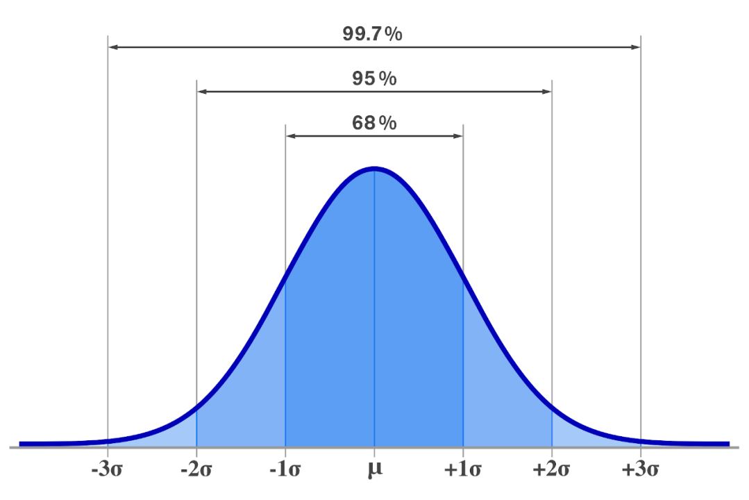
From this point forward, we make a few key simplifying assumptions that are not rigorous, but nonetheless showcase the intuition behind the problem well. Approximate \(\mathbb{P}(X_{2n}=\mathbf{0})\approx \left(\frac{d}{\sqrt{2n}}\right)^d\), by utilizing the fact that most of the probability mass for normal distributions lie within one standard deviation of the mean. This approximation will be used from here to show that the origin is a transient state for \(d>2\) and a recurrent state otherwise.
Showing Recurrence and Transience
Recall that the origin is recurrent if and only if \(\mathbb{E}\left[\sum_{n=1}^\infty\mathbb{1}\{X_{2n}=0\}\right]=\infty\). Since \(\mathbb{E}[\mathbb{1}\{A\}]=\mathbb{P}(A)\), we have
\[\mathbb{E}\left[\sum_{n=1}^\infty\mathbb{1}\{X_{2n}=0\}\right]=\sum_{n=1} ^\infty\mathbb{P}(X_{2n}=0)\approx\sum_{n=1} ^\infty\left(\frac{d}{\sqrt{2n}}\right)^d=\frac{d ^d}{2 ^{d/2}}\sum_{n=1} ^\infty n ^{-d/2}\]
For \(d=1,2\), we have that \(\sum_{n=1} ^\infty n ^{-d/2}=\infty\), but for \(d>2\), we have that \(\sum_{n=1} ^\infty n ^{-d/2}<\infty\). Thus, we have explained the perplexing property of multi-dimensional random walks.
References
The following sources of information were used in the creation of this blog post:
- Why do random walks get lost in 3D? (Ari Seff)
- Random walks in 2D and 3D are fundamentally different (Markov chains approach) (Mathemaniac)
- Markov Chains (EECS 126, UC Berkeley)